Theoretical Evolutionary Genetics is at the heart of evolutionary biology. Francis Galton and his followers laid the foundations of theoretical evolution soon after Darwin’s Origin. This so-called biometrics school had its continuity in the work of Ronald Fisher, who amalgamated the Biometric and Mendelian schools into a robust theoretical framework. Animal breeders such as Sewall Wright independently developed methods to study heredity and genetic improvement in animal stocks. Fisher, Wright and Haldane (the latter coming from a different tradition, his own) are acknowledged to be the founding fathers of population genetics.
The fact that population genetics is the basis of theoretical evolutionary biology may be seen as an accident of the way it was introduced by the founding trio. As a matter of fact, there are ways of exploring the same biological problems other than the canonical population genetics approach. I recently bought two textbooks on evolution and I found that they used completely different approaches. After I read them I became aware that, indeed, there are at least three ways of doing things in theoretical evolutionary biology. These are the three ‘flavours’:
Flavour 1: Standard Population Genetics
This flavour is best represented by the Crow and Kimura manual, and more recently by the Charlesworths’ textbook. Evolutionary problems are tackled from the point of view of evolving populations in which allele frequencies change as a function of their relative selective fitness and sampling effects. Typically, a ‘change in allele frequency’ is defined and the resulting equation is solved for specific cases. These cases are basically equilibria situations or, in case of fixation/losses of alleles, how long will the process take and with which probability (on average). OK, this is an extreme oversimplification of population genetics, but for what I want to say it’s enough.
Flavour 2: Price’s Equation
I must admit that I never got Price’s equation. I mean, even after someone explained it to me and I thought I understood it, I didn’t see what it was useful for. I have recently changed my mind. I recently read Sean Rice’s ‘Evolutionary Theory’ and see, to my astonishment, that he approached classic problems in population biology using Price’s equation. Price’s equation is due to George Price, a strange man and even stranger scientist. He wrote down the whole evolutionary process into a single equation, accounting for the fitness of the ‘elements’ of an evolutionary system and the relationships between these elements (species, genes…). It’s basically a covariance equation. Using the appropriate definition of parameters one can reduce complex population genetics problems into a single covariance equation, and that’s the strength of Price’s approach.
Flavour 3: Game Theory

Game theory was used in biology originally by Bill Hamilton (I think) although it was definitively John Maynard Smith who fully developed the topic. According to Maynard Smith, he started using Game Theory while visiting Chicago, as there was nothing else to do in Chicago! Anyway, I always thought that game theory was useful for phenotype evolution modelling (like behaviour). However, while reading Martin Nowak’s ‘Evolutionary Dynamics’ I discovered that most of what we know from standard population genetics could be approached from the game theory perspective. In that case different alleles represent different game strategies. Winning strategies are equivalent to fitter alleles and the winner of the game is, obviously, the fixed allele in the population.
Is there a best flavour?
I should say that my preferred method is that of classical canonical standard population genetics, but after reading Nowak’s and Rice’s books I’m aware that this is only a personal preference. What these different approaches show is that there are many ways of solving the same problem, and that should be used as a powerful tool in evolutionary biology. As an example, I included a BOX below in which I derive a classical result in population genetics using these three different approaches. Richard Levins once wrote that “[deriving] alternative proofs for the same result is not merely a mathematical exercise – it is a method of validation”. Now I wonder whether all major findings in population genetics achieved during the last century could be reproduced by using these alternative flavours!
Box 1. Deriving the change in allele frequency with three different approaches.
One of the most important quantities in population genetics is how much an allele frequency changes after one generation, or 


Standard approach
The change in an allele frequency for an haploid population is given by (Crow and Kimura 1970):

where 


being 

For a small 

obtaining the classic result for haploid populations:

Price’s equation approach
A common form of Price’s equation is (Rice 2004):
![\Delta \overline{\Phi} = \dfrac{1}{\overline{w}}[cov(w,\Phi) + E(w\overline{\delta})]](https://s0.wp.com/latex.php?latex=%5CDelta+%5Coverline%7B%5CPhi%7D+%3D+%5Cdfrac%7B1%7D%7B%5Coverline%7Bw%7D%7D%5Bcov%28w%2C%5CPhi%29+%2B+E%28w%5Coverline%7B%5Cdelta%7D%29%5D+&bg=cccccc&fg=333333&s=0&c=20201002)
and it says that the change in a trait or character (


![\Delta \overline{\Phi} = \dfrac{1}{\overline{w}}[\overline{\Phi}(w-\overline{w})]](https://s0.wp.com/latex.php?latex=%5CDelta+%5Coverline%7B%5CPhi%7D+%3D+%5Cdfrac%7B1%7D%7B%5Coverline%7Bw%7D%7D%5B%5Coverline%7B%5CPhi%7D%28w-%5Coverline%7Bw%7D%29%5D+&bg=cccccc&fg=333333&s=0&c=20201002)
As we are interested in the allele frequency as a trait we rewrite this formula in a more familiar form:
![\Delta p = \dfrac{1}{\overline{w}}[p(w_1-\overline{w})]](https://s0.wp.com/latex.php?latex=%5CDelta+p+%3D+%5Cdfrac%7B1%7D%7B%5Coverline%7Bw%7D%7D%5Bp%28w_1-%5Coverline%7Bw%7D%29%5D+&bg=cccccc&fg=333333&s=0&c=20201002)
which for the selection scheme defined above is equivalent to:

which to a linear approximation leads to the same result as the classic approach:

Game theory approach
Last but not least, we can consider that the two alleles are two strategies in a game played by their bacterial hosts. In game theory we first create a table of costs of the different strategies like this one:

In our case, if two bacteria play the same strategy (they have the same allele) there is no cost or benefit for any of them. However, if one bacteria has the fitter allele while the other has the alternative allele, the benefit for one will be the selection coefficient 

The instant rate of change of the winning strategy frequency is given by (Nowak 2006):
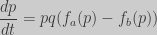
For our game we have:


So that:

moving 

and for a time interval of one generation (


In conclusion, the three different approaches based on different assumptions yield the same result.


